The body of data on COVID-19 grows daily, and with it, the scope of possible data-driven conclusions that could be drawn from it. In this article I describe how I used the SKLearn open source Machine Learning library and the COVID19 Dataset from the Royal Society DELVE Initiative to try and understand why some countries have been more affected than others and how the implementation of certain measures may have helped. The Royal Society DELVE initiative has put together a global dataset on COVID19. The dataset has been consolidated from multiple sources and includes 62 fields for each country that range from the weather, Non Pharmaceutical Interventions (NPI) to Case, Test and Mobility numbers.
This article continues on from COVID19 Dataset from the Royal Society DELVE Initiative where we explored the dataset and looked at how various parameters and interventions affected the number of cases.
Machine Learning is a subset of artificial intelligence that allows a computer to learn and make predictions without being explicitly programmed to do so. A machine learning model is trained by feeding it data that has a correct answer attached. This training data allows the model to connect patterns in the data to the correct answer. Once the model has been trained it can be given test data that has no answers attached. The model then predicts the answers based on the training it received.
I have used a Support Vector Machine Regression (SVMR) model to predict new cases per day from some of the fields in the dataset.
It is worth noting that I used cases_total in the training data and this was to tether the model to reality so that when changes are made to the data, for example to the face mask policy, that one change should not have a large effect on the predictions unless that change is significant. Put another way because there is a direct correlation between new cases per day and total cases including that field in the training data will effectively make it more difficult for any other field to change the predicted number of cases per day.
The fields used in the training data were.
- DATE
- npi_school_closing
- npi_workplace_closing
- npi_cancel_public_events
- npi_gatherings_restrictions
- npi_close_public_transport
- npi_stay_at_home
- npi_internal_movement_restrictions
- npi_international_travel_controls
- npi_income_support
- npi_debt_relief
- npi_fiscal_measures
- npi_international_support
- npi_public_information
- npi_testing_policy
- npi_contact_tracing
- npi_healthcare_investment
- npi_vaccine_investment
- npi_stringency_index
- npi_masks
- cases_total
- tests_total
- tests_new
- tests_total_per_thousand
- tests_new_per_thousand
- tests_new_smoothed
- tests_new_smoothed_per_thousand
- stats_population
- stats_population_density
- stats_median_age
- stats_gdp_per_capita
- mobility_retail_recreation
- mobility_grocery_pharmacy
- mobility_parks
- mobility_transit_stations
- mobility_workplaces
- mobility_residential
- mobility_travel_driving
- mobility_travel_transit
- mobility_travel_walking
- stats_hospital_beds_per_1000
- stats_smoking
- stats_population_urban
- stats_population_school_age
- weather_precipitation_mean
- weather_humidity_mean
- weather_sw_radiation_mean
- weather_temperature_mean
- weather_temperature_min
- weather_temperature_max
- weather_wind_speed_mean
These fields were not used.
- deaths_total
- deaths_new
- cases_total_per_million
- cases_new_per_million
- deaths_total_per_million
- deaths_new_per_million
- deaths_excess_daily_avg
- deaths_excess_weekly
- cases_days_since_first
- deaths_days_since_first
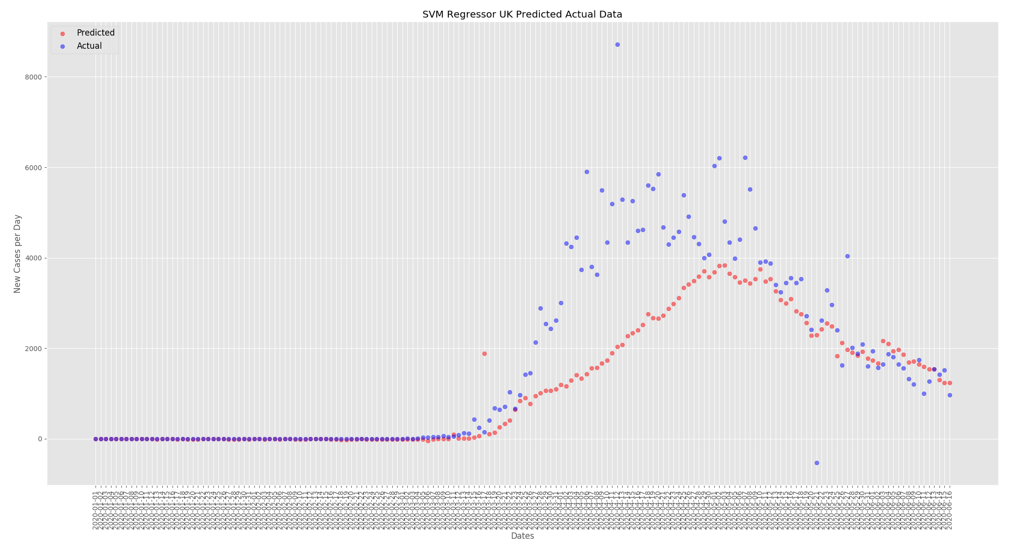
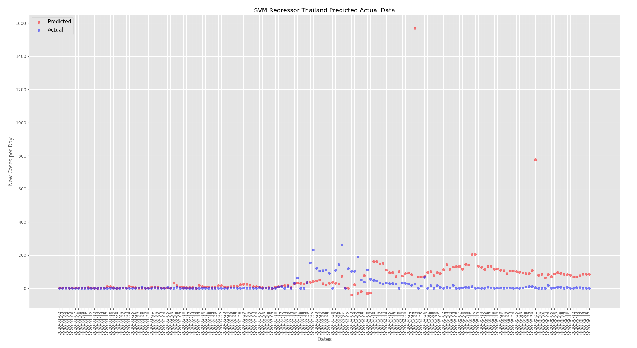
New cases per day were predicted for the UK and Thailand. When making predictions for the UK all other countries except the UK were used to train the model and when making predictions for Thailand all other countries except Thailand were used to train the model. Nothing was changed in the data, this is a look at how well the model can predict new cases per day based on the actual data for the UK and Thailand.
The graphs below show the predictions from the SVMR based on the actual data for the UK and Thailand. For both countries the predictions are fairly close to what actually happened the predictions are a little low at the beginning of the outbreak but start to converge towards the end.
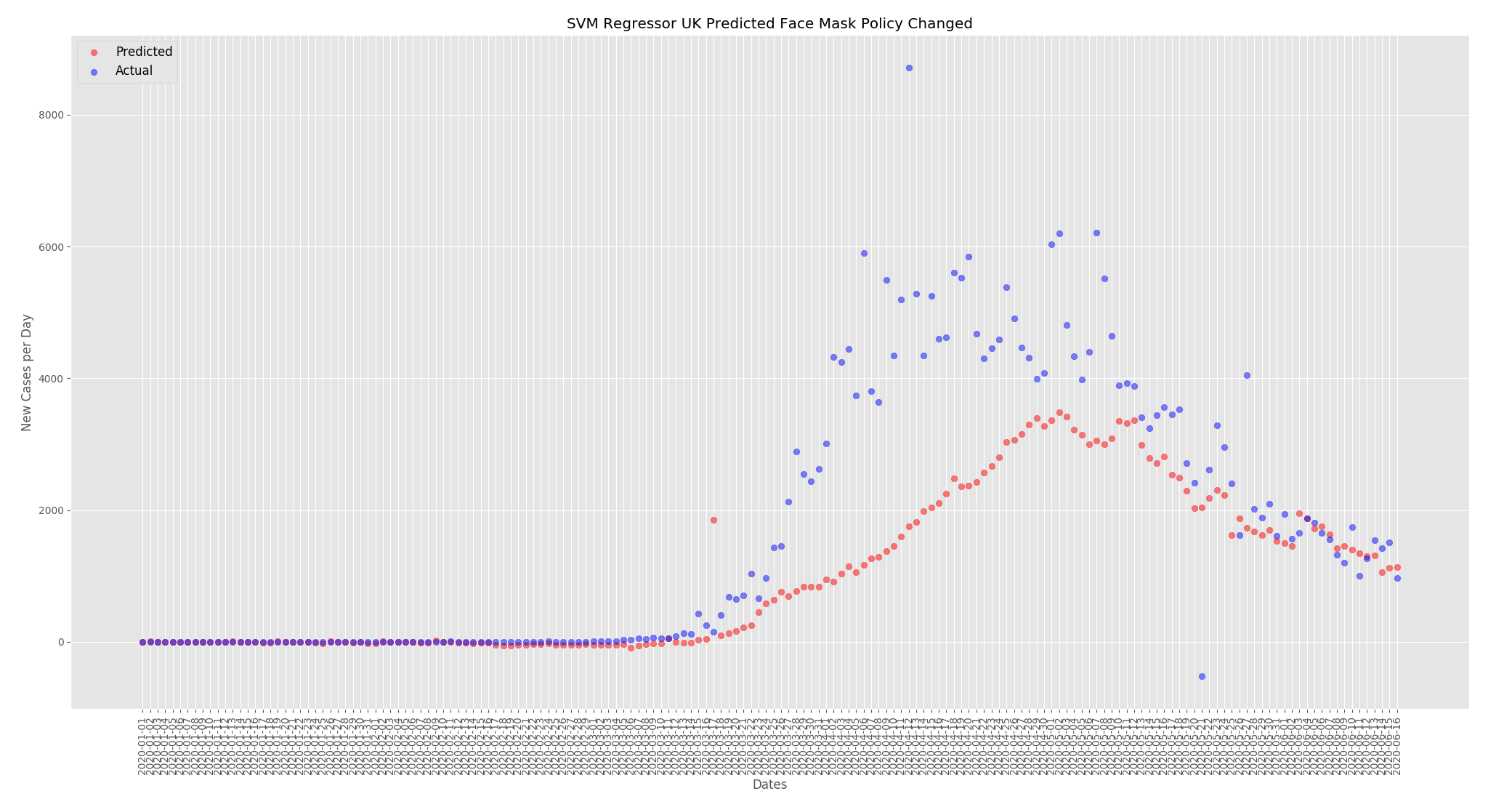
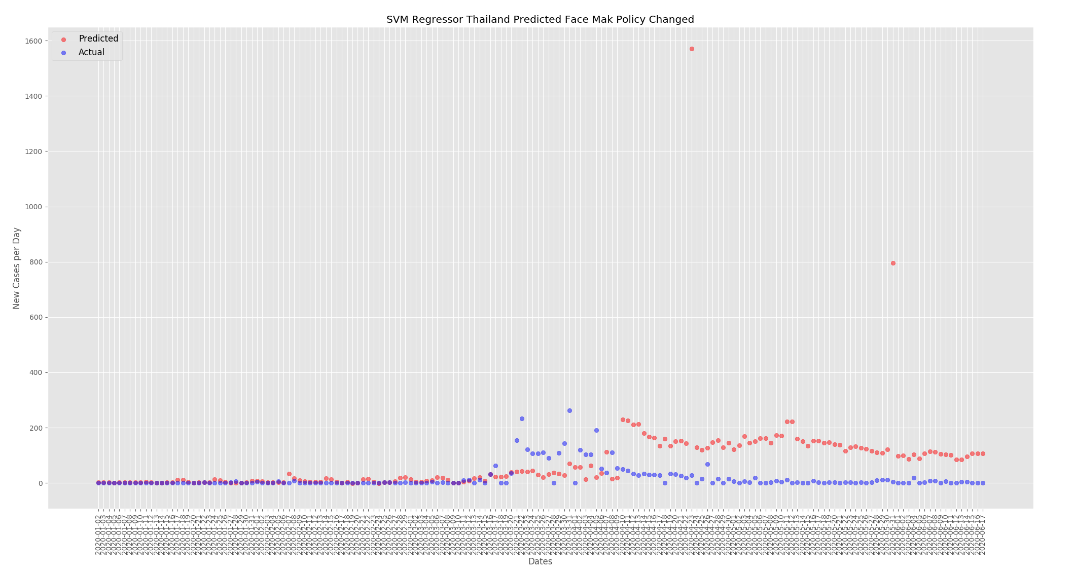
Now that we have a baseline I wanted to look at how face mask use and temperature can affect the predicted new cases per day. For these predictions I changed the UK face mask policy to mandatory everywhere and changed the humidity and temperatures to be comparable, but not the same, as Thailand. For Thailand I did the opposite and changed the face mask policy to none and reduced the temperatures and humidity to be similar but not the same as the UK.
The graphs below show the effect of changing the face mask policies. For the UK the predicted new cases per day has decreased. When compared to the predictions from the actual data above the numbers have dropped from around 4000 at the peak to around 3500.
For Thailand the predicted new cases per day has increased. When compared to the predictions from the actual data above the numbers have increased from around 125 to around 180.
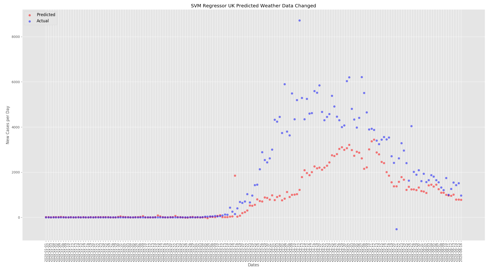
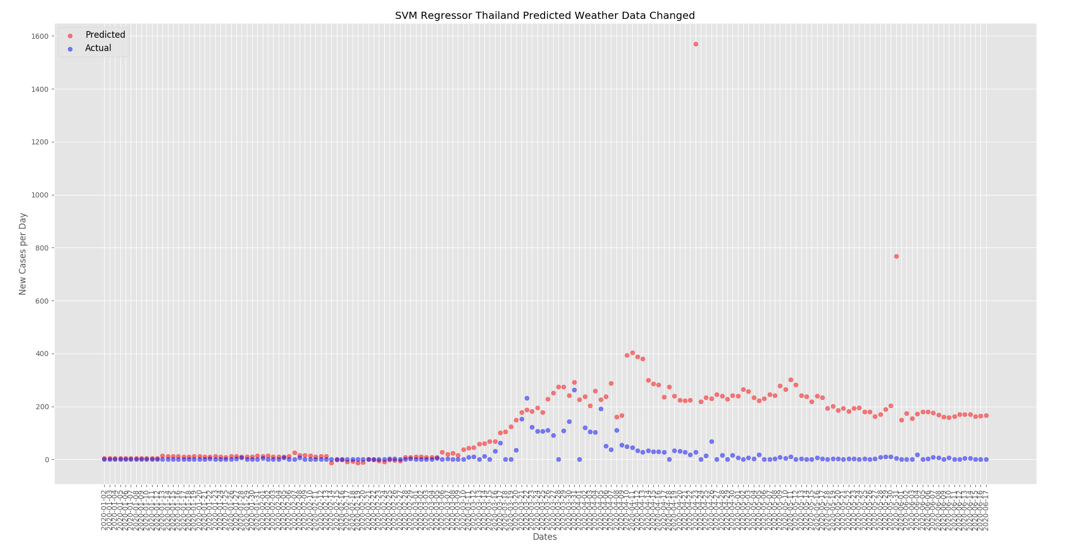
The graphs below show the effect of changing the weather as detailed above. For the UK the predicted new cases per day has decreased. When compared to the predictions from the actual data the numbers have dropped from around 4000 at the peak to around 3250.
For Thailand the predicted new cases per day has increased. When compared to the predictions from the actual data above the numbers have increased from around 125 to around 225.
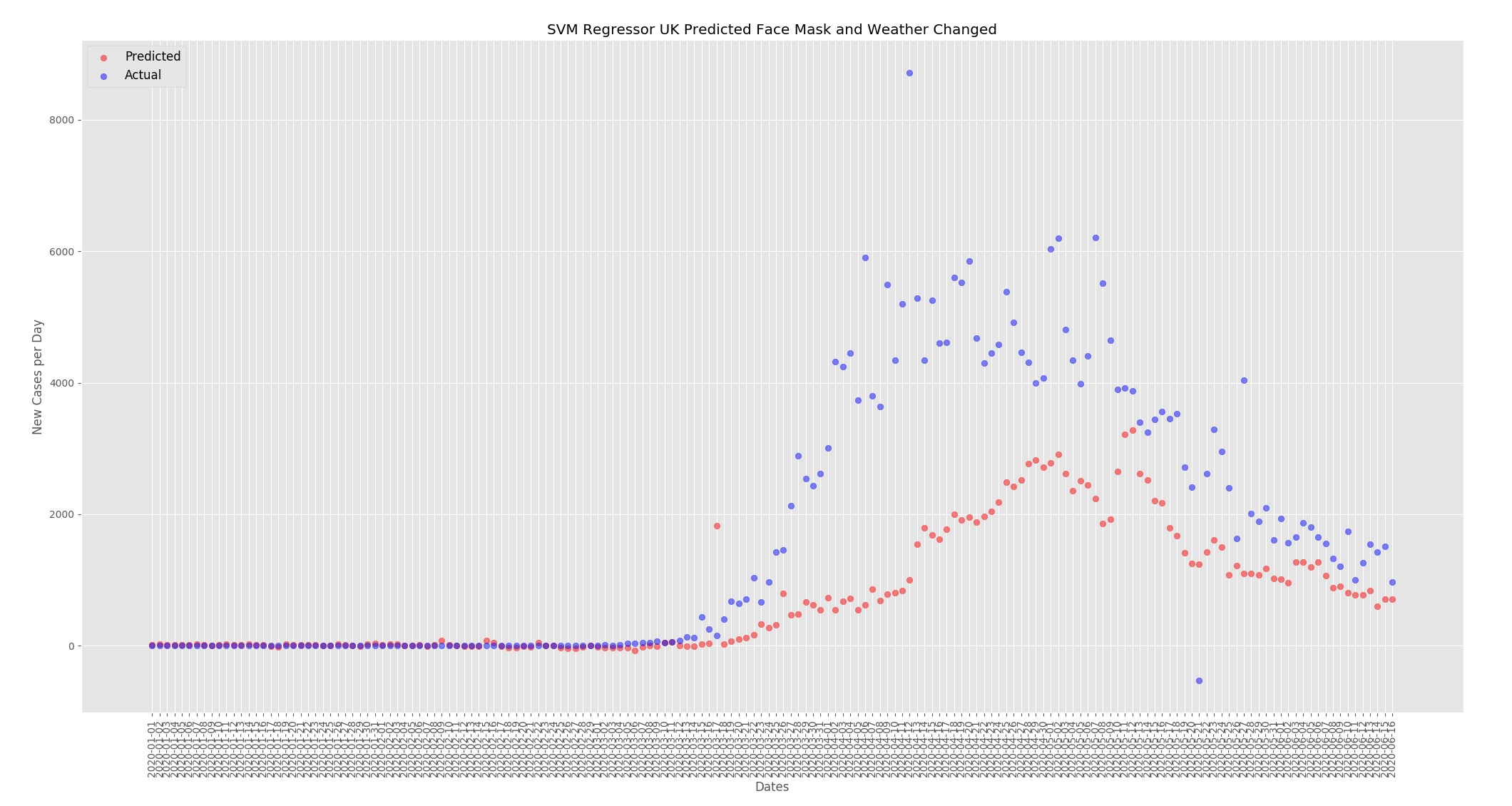
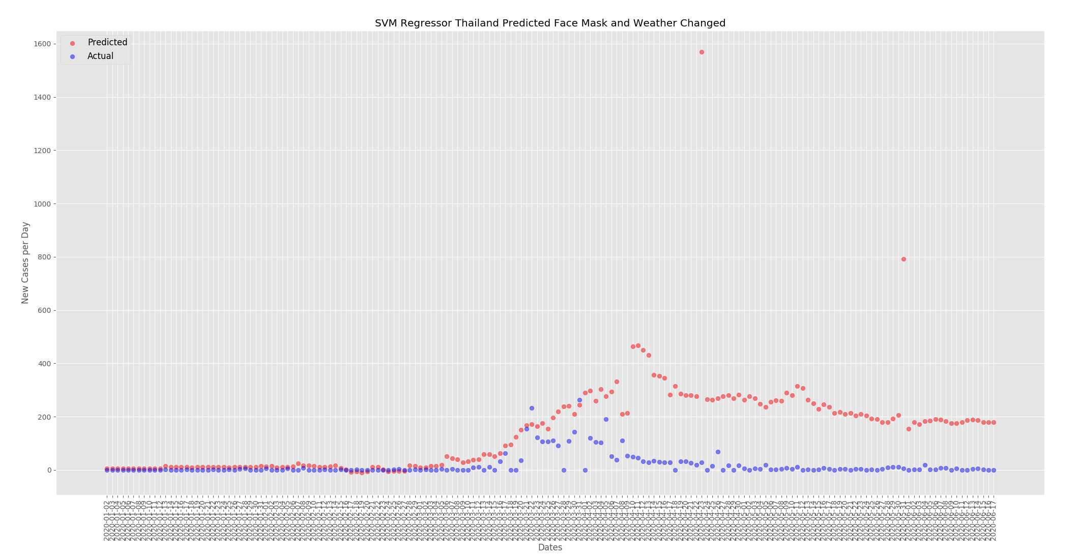
The graphs below show the effect of changing the weather and the face mask policy as detailed above. For the UK the predicted new cases per day has decreased. When compared to the predictions from the actual data the numbers have dropped from around 4000 at the peak to around 3000.
For Thailand the predicted new cases per day has increased. When compared to the predictions from the actual data above the numbers have increased from around 125 to around 300.
There may be other factors at play but I believe this data set shows that face mask use and temperature and humidity have an effect on the number of cases. As outlined above I included the total cases in the training data to help suppress any changes in the predictions as the face mask policy and weather was changed. But when the temperature and humidity was increased for the UK the numbers went down. When the face mask policy was changed to mandatory everywhere for the UK the numbers also went down. The opposite happened for Thailand where when the weather was changed to be similar to the UK, cold and dry, the numbers went up and when the face mask policy was changed to none the numbers went up.
Python 3.7 Support Vector Machine Regression
import numpy as np
import matplotlib.pyplot as plt
from sklearn import svm, preprocessing
import pandas as pd
from matplotlib import style
import math
from sklearn.model_selection import TimeSeriesSplit,GridSearchCV,train_test_split
from sklearn.metrics import mean_squared_error, r2_score
from sklearn.metrics import make_scorer
import datetime as dt
from sklearn import neighbors
from sklearn.tree import DecisionTreeRegressor
from sklearn.ensemble import RandomForestRegressor
style.use("ggplot")
# Did not use these features,
#'deaths_total', 'deaths_new', 'cases_total_per_million', 'cases_new_per_million', 'deaths_total_per_million', 'deaths_new_per_million','deaths_excess_daily_avg', 'deaths_excess_weekly', 'cases_days_since_first', 'deaths_days_since_first',
FEATURES = [
'DATE','npi_school_closing', 'npi_workplace_closing', 'npi_cancel_public_events', 'npi_gatherings_restrictions','npi_close_public_transport',
'npi_stay_at_home', 'npi_internal_movement_restrictions', 'npi_international_travel_controls','npi_income_support','npi_debt_relief', 'npi_fiscal_measures',
'npi_international_support', 'npi_public_information', 'npi_testing_policy', 'npi_contact_tracing', 'npi_healthcare_investment', 'npi_vaccine_investment',
'npi_stringency_index', 'npi_masks', 'cases_total', 'tests_total', 'tests_new', 'tests_total_per_thousand', 'tests_new_per_thousand', 'tests_new_smoothed', 'tests_new_smoothed_per_thousand',
'stats_population', 'stats_population_density','stats_median_age', 'stats_gdp_per_capita', 'mobility_retail_recreation', 'mobility_grocery_pharmacy',
'mobility_parks', 'mobility_transit_stations', 'mobility_workplaces', 'mobility_residential', 'mobility_travel_driving', 'mobility_travel_transit', 'mobility_travel_walking',
'stats_hospital_beds_per_1000','stats_smoking', 'stats_population_urban', 'stats_population_school_age', 'weather_precipitation_mean', 'weather_humidity_mean',
'weather_sw_radiation_mean','weather_temperature_mean', 'weather_temperature_min','weather_temperature_max','weather_wind_speed_mean'
]
def Build_Data_Set():
data_df = pd.read_csv("combined_dataset_latest-ukmod.csv")
dates = (data_df["DATE"].values.tolist())
data_df['DATE'] = pd.to_datetime(data_df['DATE'])
data_df['DATE']= (data_df['DATE'] - dt.datetime(1970,1,1)).dt.total_seconds()
scaler = preprocessing.StandardScaler()
data_df[['DATE', 'npi_school_closing', 'npi_workplace_closing', 'npi_cancel_public_events', 'npi_gatherings_restrictions','npi_close_public_transport',
'npi_stay_at_home', 'npi_internal_movement_restrictions', 'npi_international_travel_controls','npi_income_support','npi_debt_relief', 'npi_fiscal_measures',
'npi_international_support', 'npi_public_information', 'npi_testing_policy', 'npi_contact_tracing', 'npi_healthcare_investment', 'npi_vaccine_investment',
'npi_stringency_index', 'npi_masks', 'cases_total', 'tests_total', 'tests_new', 'tests_total_per_thousand', 'tests_new_per_thousand', 'tests_new_smoothed', 'tests_new_smoothed_per_thousand',
'stats_population', 'stats_population_density','stats_median_age', 'stats_gdp_per_capita', 'mobility_retail_recreation', 'mobility_grocery_pharmacy',
'mobility_parks', 'mobility_transit_stations', 'mobility_workplaces', 'mobility_residential', 'mobility_travel_driving', 'mobility_travel_transit', 'mobility_travel_walking',
'stats_hospital_beds_per_1000','stats_smoking', 'stats_population_urban', 'stats_population_school_age', 'weather_precipitation_mean', 'weather_humidity_mean',
'weather_sw_radiation_mean','weather_temperature_mean', 'weather_temperature_min','weather_temperature_max',
'weather_wind_speed_mean']] = scaler.fit_transform(data_df[['DATE', 'npi_school_closing', 'npi_workplace_closing', 'npi_cancel_public_events', 'npi_gatherings_restrictions',
'npi_close_public_transport','npi_stay_at_home', 'npi_internal_movement_restrictions', 'npi_international_travel_controls','npi_income_support','npi_debt_relief', 'npi_fiscal_measures',
'npi_international_support', 'npi_public_information', 'npi_testing_policy', 'npi_contact_tracing', 'npi_healthcare_investment', 'npi_vaccine_investment',
'npi_stringency_index', 'npi_masks', 'cases_total', 'tests_total', 'tests_new', 'tests_total_per_thousand', 'tests_new_per_thousand', 'tests_new_smoothed', 'tests_new_smoothed_per_thousand',
'stats_population', 'stats_population_density','stats_median_age', 'stats_gdp_per_capita', 'mobility_retail_recreation', 'mobility_grocery_pharmacy',
'mobility_parks', 'mobility_transit_stations', 'mobility_workplaces', 'mobility_residential', 'mobility_travel_driving', 'mobility_travel_transit', 'mobility_travel_walking',
'stats_hospital_beds_per_1000','stats_smoking', 'stats_population_urban', 'stats_population_school_age', 'weather_precipitation_mean', 'weather_humidity_mean', 'weather_sw_radiation_mean',
'weather_temperature_mean', 'weather_temperature_min','weather_temperature_max','weather_wind_speed_mean']])
#Shuffled data when tuning
#data_df = data_df.reindex(np.random.permutation(data_df.index))
#data_df.fillna(data_df.mean(), inplace=True)
data_df.fillna(0, inplace=True)
X = np.array(data_df[FEATURES].values)
y = (data_df["cases_new"].values.tolist())
#Split the data for training and test
## X_train, X_test, y_train, y_test = train_test_split(X,y, test_size=0.2, shuffle=True, random_state=42)
## X_train = preprocessing.scale(X_train)
## X_test = preprocessing.scale(X_test)
X = preprocessing.scale(X)
return X,y,dates
def Analysis():
test_size = 169
X, y, dates = Build_Data_Set()
## #Tuning
## parameters = [{'kernel': ['rbf'], 'epsilon': [0.01, 0.1, 3, 5], 'gamma': [0.00001,0.005,0.01,0.02],'C': [100,1000,5000]}]
## scorer = make_scorer(mean_squared_error, greater_is_better=False)
## print("Tuning hyper-parameters")
## svr = GridSearchCV(svm.SVR(), parameters, cv = 3, scoring=scorer, n_jobs=-1)
## svr.fit(X, y)
##
## # Checking the score for all parameters
## print("Grid scores on training set:")
## means = svr.cv_results_['mean_test_score']
## stds = svr.cv_results_['std_test_score']
## for mean, std, params in zip(means, stds, svr.cv_results_['params']):
## print("%0.3f (+/-%0.03f) for %r"% (mean, std * 2, params))
regr = svm.SVR(kernel='rbf', C=1000, gamma=0.01, epsilon=0.1)
regr.fit(X[:-test_size],y[:-test_size])
#KNN_ = neighbors.KNeighborsRegressor(algorithm='kd_tree', leaf_size=120, p=10, n_neighbors=500, weights='distance').fit(X[:-test_size],y[:-test_size])
#dtree = DecisionTreeRegressor()
#dtree.fit(X[:-test_size],y[:-test_size])
#model_rf = RandomForestRegressor(n_estimators=1000)
#model_rf.fit(X[:-test_size],y[:-test_size])
correct_count = 0
predictions_list = []
actuals_list = []
dates_list = []
pred_total=0
for x in range(1, test_size+1):
predictions = regr.predict([X[-x]])
#predictions = KNN_.predict([X[-x]])
#predictions = dtree.predict([X[-x]])
#predictions= model_rf.predict([X[-x]])
#error = predictions-y[-x]
#print(error)
print("The Prediction ", predictions)
print("The Actual ", y[-x])
predictions_list.append(math.floor(predictions[0]))
pred_total += math.floor(predictions[0])
actuals_list.append(y[-x])
dates_list.append(dates[-x])
allowed_error = y[-x] * 0.2
if abs(predictions) <= 5 and y[-x] <= 5:
correct_count += 1
elif abs(predictions - y[-x]) <= allowed_error:
correct_count += 1
predictions_list.reverse()
actuals_list.reverse()
dates_list.reverse()
print("Accuracy:", (correct_count/test_size) * 100.00)
print("Total Predictions", pred_total)
print("R2 score : %.2f" % r2_score(actuals_list,predictions_list))
print("Mean squared error: %.2f" % mean_squared_error(actuals_list,predictions_list))
er = []
g = 0
for i in range(len(actuals_list)):
print( "actual=", actuals_list[i], " observed=", predictions_list[i])
x = (actuals_list[i] - predictions_list[i]) **2
er.append(x)
g = g + x
x = 0
for i in range(len(er)):
x = x + er[i]
print ("MSE", x / len(er))
v = np.var(er)
print ("variance", v)
print ("average of errors ", np.mean(er))
m = np.mean(actuals_list)
print ("average of observed values", m)
y = 0
for i in range(len(actuals_list)):
y = y + ((actuals_list[i] - m) ** 2)
print ("total sum of squares ", y)
print ("ẗotal sum of residuals ", g)
print ("r2 calculated", 1 - (g / y))
plt.xticks(rotation=90)
predg = plt.scatter(dates_list, predictions_list, c='red', alpha=0.5)
actg = plt.scatter(dates_list, actuals_list, c='blue', alpha=0.5)
plt.legend((predg, actg),
('Predicted', 'Actual'),
scatterpoints=1,
loc='upper left',
ncol=1,
fontsize=12)
plt.title("UK Predicted per Day)
plt.xlabel("Dates")
plt.ylabel("New Cases per Day")
plt.show()
Analysis()