1.0 Summary
The UNSW-NB15 data set is a benchmark that can be used to test Network Anomaly Detection Systems. It contains normal network traffic and nine types of attacks both represented by forty- nine features extracted from network traffic flow. In the paper The evaluation of Network Anomaly Detection Systems: Statistical analysis of the UNSW-NB15 data set and the comparison with the KDD99 data-set (hereinafter referred to as the Evaluation Paper), the authors demonstrate the complexity of UNSW-NB15 using three approaches; statistical analysis, feature correlation and five machine learning models (Moustafa & Slay 2016). The results are compared to an older benchmark, namely the KDDCUP1999 data set which does not include modern types of attacks nor network traffic flows (KDDCUP1999 2007).
In addition to repeating the analysis carried out in the Evaluation Paper a Support Vector Machine (SVM) and a Neural Network (NN) model both with tuned parameters are implemented to increase the accuracy and decrease the False Alarm Rate (FAR) of the predictions.
The results obtained agree with those presented in the Evaluation Paper and confirm that the UNSW-NB15 data set is more complex than the KDDCUP1999 data set. Further both the tuned SVM and NN show very high accuracies but there are still an unacceptable number of false positives and negatives.
2.0 Introduction
The aim of this work is to repeat the analysis carried out in the Evaluation Paper and extend it by tuning a Support Vector Machine (SVM) and a Neural Network (NN) model to increase the accuracy and decrease the False Alarm Rate (FAR).
The three approaches used in the Evaluation Paper were statistical analysis, feature correlation analysis and five machine learning model implementations.
The statistical analysis methods were performed with the SPSS tool and include:
i. Kolmogorov–Smirnov (K-S) test
ii. Multivariate Skewness
iii. Multivariate Kurtosis
The correlation methods were performed with SPSS, MatLab and Python and include:
i. Pearson Correlation Coefficient (PCC)
ii. Gain Ratio
The machine learning models were implemented with SQL Server and Visual Studio and include: i. i. Naïve Bayes (NB)
ii. Decision Tree (DT)
iii. Neural Network (NN)
iv. Logistic Regression (LR)
v. Clustering
The new SVM was implemented in R and the NN was implemented with SQL Server and Visual Studio.
This paper is organised as follows: Section 3.0 Approach outlines the data sets, features and pre-processing used in the analysis. Section 3.1 Statistical Analysis details the statistical tests performed and Section 3.2 Feature Correlation Analysis outlines the PCC and Gain Ratio tests. Section 3.3 Machine Learning implements the models reported in the Evaluation Paper and Section 3.4 details the tuned SVM and NN Models. The results are presented in Section 4.0 and the conclusions are discussed in Section 5.0.
3.0 Approach
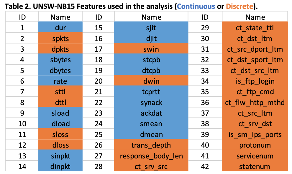
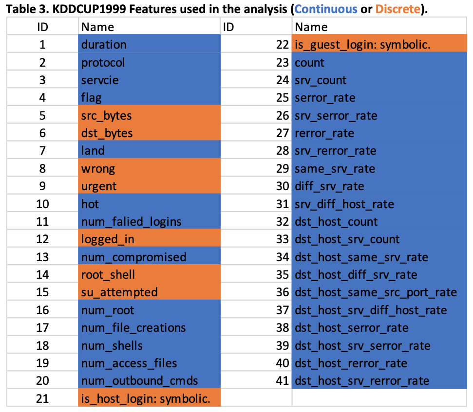
There are three features in all of the data sets detailed in Table 1 that are represented by character strings, these features were mapped to integers using the SPSS Transform > Automatic Recode tool (SPSS tool 2020). Specifically, the features mapped are protonum, servicenum and statenum in the UNSW-NB15 data sets and protocol, service and flag features in the KDDCUP1999 data sets, please see Tables 2 and 3. These mapped features were used in all of the statistical analysis’, feature correlations and machine learning models.
Further because the features in the data sets have a large distance between the minimum and maximum values, they were standardized using the Z-Score tool in SPSS, specifically with Analyze > DescriptiveStatistics > Descriptive and using the Save standardised values as variables option.

3.1 Statistical Analysis
The SPSS tool (SPSS tool 2020) was used to analyze the UNSW-NB15 Training and Testing data sets (Moustafa 2018). Table 1 and Table 2 detail the records and features for both the sets. The three techniques used were the Kolmogorov–Smirnov (K-S) test, Multivariate Skewness and Multivariate Kurtosis.
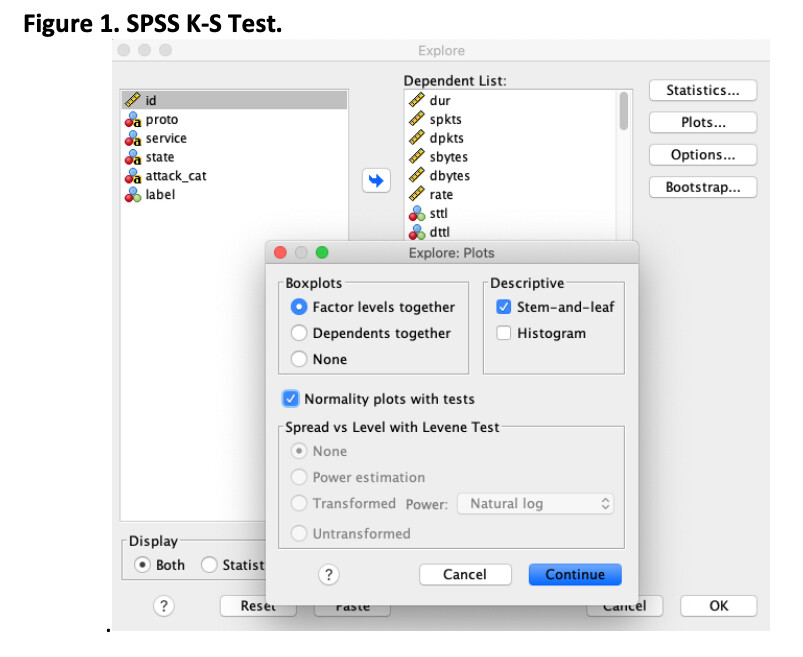
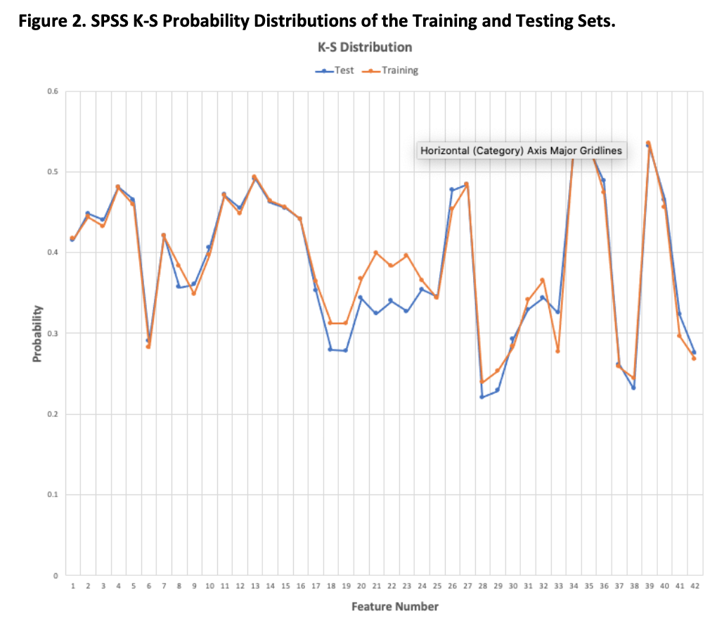
3.1.0 The K-S test is used to compare the probability distributions of the features in the training and testing sets. The results obtained by using the SPSS tool Analyze > DescriptiveStatistics > Explore and Normality plots with tests, agree with those presented in the Evaluation Paper. This illustrates that the probability distributions of the features in the training and testing sets show a strong similarity. Please see Figures 1 and 2 below and Appendix D for the full list of results.
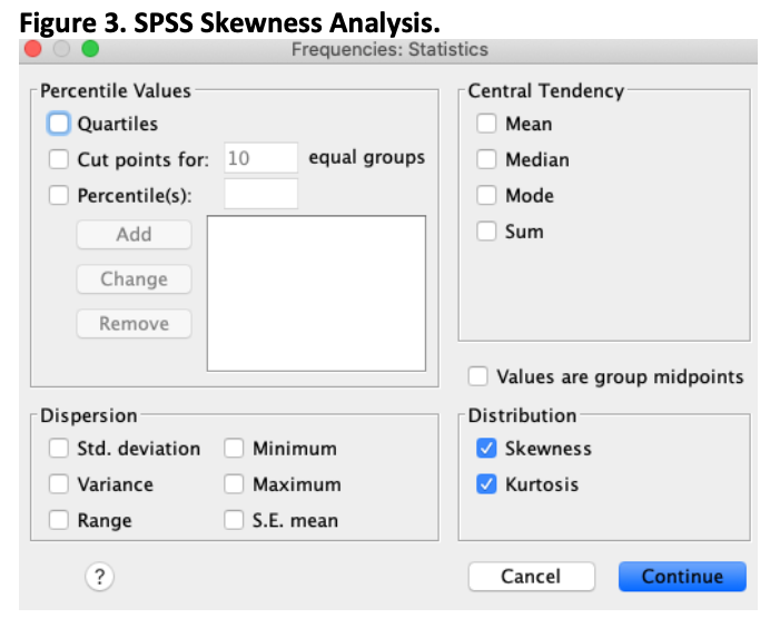
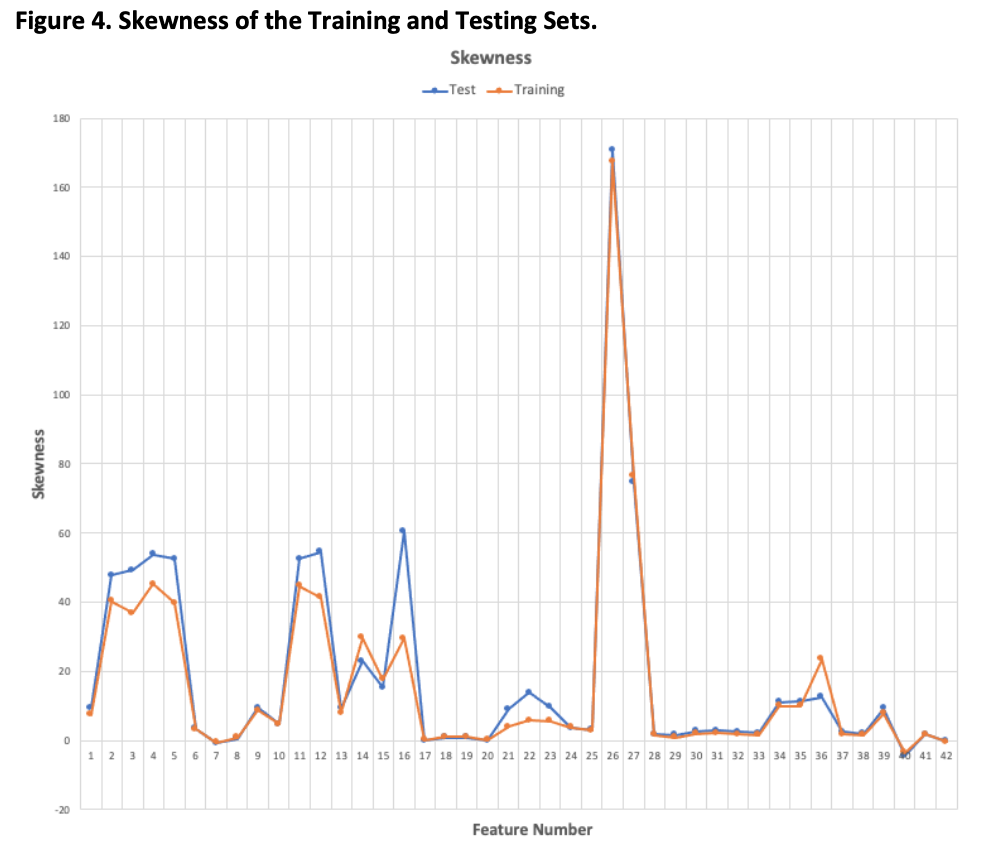
3.1.1 The Multivariate Skewness analysis is used to measure the asymmetry of the feature distributions and was performed with SPSS, specifically using Analyze > Frequencies > Distribution > Skewness and Kurtosis. The results obtained match those presented in the Evaluation Paper. The results show that the training and testing set features have very similar distributions with only the sttl feature having a negative skewness in both sets. The swin and dwin features in the training set show a very slight negative skewness and the trans_depth and response_body_length are very positively skewed. Please see Figures 3 and 4 below and Appendix D for the full list of results.
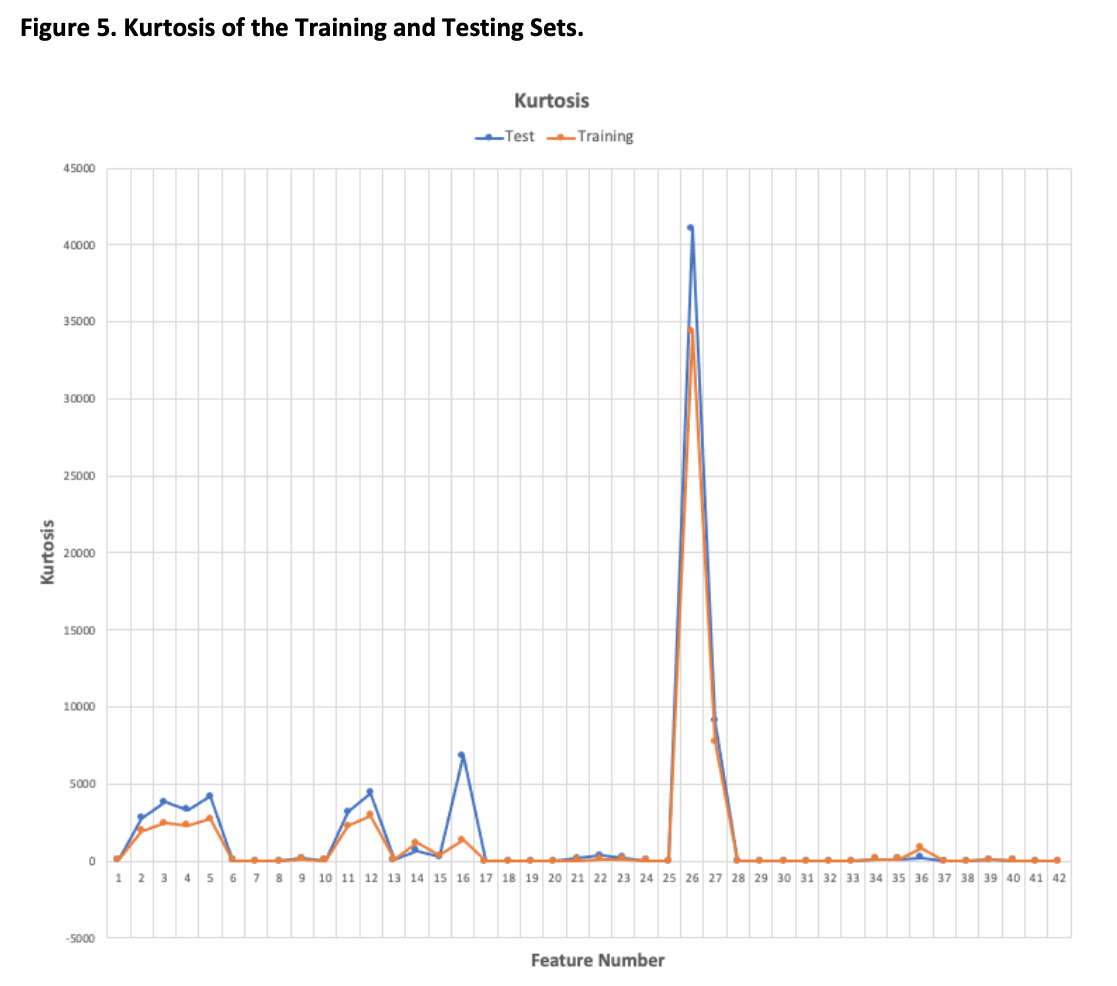
3.1.2 The Multivariate Kurtosis analysis is used to measure how extreme the tails of the feature distributions are and was performed with SPSS as per section 3.1.1. The results obtained agree with those presented in the Evaluation Paper. The high Kurtosis values indicate a large number of outliers and low Kurtosis values indicate a lack of outliers. The trans_depth and response_body_length in both the testing and training sets have a large number of outliers while djit in the testing set has a moderate number of outliers. Some other features also have some outliers but importantly these are present in both the testing and training sets. Please see Figure 5 below and Appendix D.
3.2 Feature Correlation Analysis
The correlation of the features in the data sets was tested using two approaches; the Pearson Correlation Coefficient was used to analyze the features without the label and Gain Ratio was used to analyse the features with the label.
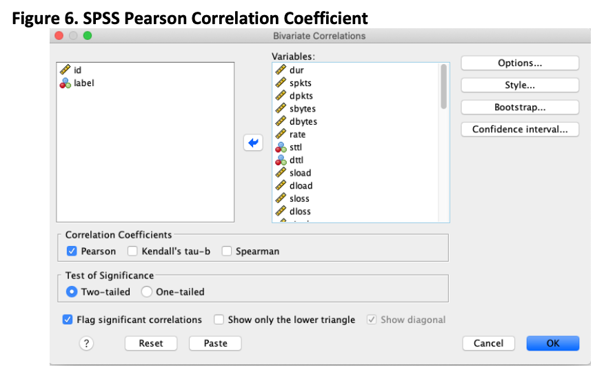
3.2.0 The Pearson Correlation Coefficient (PCC) was used to measure the correlation between the features with SPSS specifically using Analyze > Correlate > Bivariate with the Pearson Correlation Coefficient ticked. Please see Figure 6.
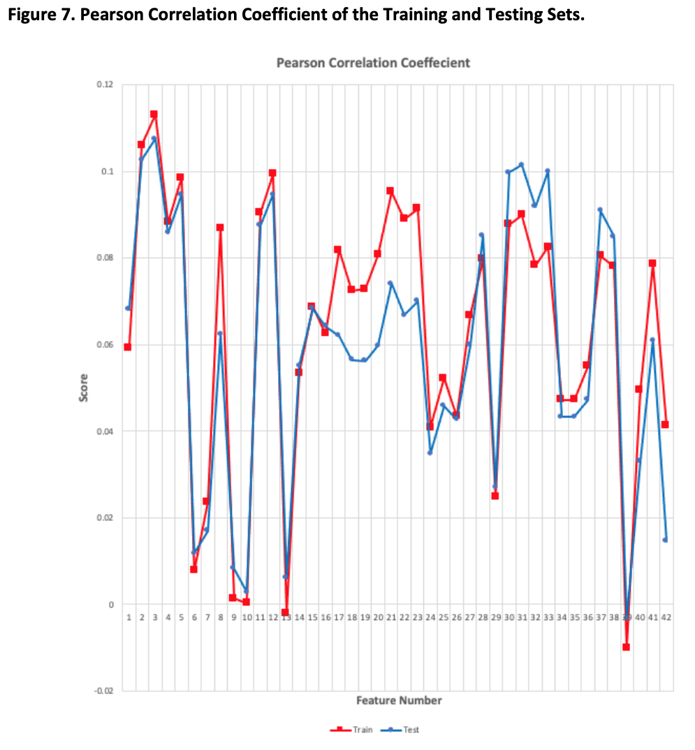
The results obtained match those presented in the Evaluation Paper. PCC is a measure of the strength of association between the features in each data set and are scored between -1 and 1. A correlation of -1 indicates an individual features average correlation with all other features is perfectly negatively linearly related. A correlation of 0 indicates an individual features average correlation with all other features does not have any linear relation. A correlation of 1 indicates an individual features average correlation with all other features is perfectly positively linearly related.
Figure 7 and Appendix D show that none of the features have a high degree of correlation with each other but this lack of correlation is shared by both the testing and training sets.
3.2.1 The Gain Ratio for an individual feature is defined as the ratio between Information Gain and Intrinsic Value. Information Gain is the measure of mutual dependence between the feature and the label where it measures the reduction in uncertainty for a given feature when the label is known. That is, a feature with a high Information Gain may just be an indication of a high number of distinct values in the feature and if that is the case this will be reflected in a low value for the Gain Ratio (Brownlee 2020).
The Gain Ratio algorithm as presented in Machine Learning: Algorithms and Applications (Mohammed, Badruddin, Bashier. 2016) was attempted with MatLab (MatLab tool 2020), but I was unable to implement it correctly. Please see Appendix A for the code snippet. The principle author of the Evaluation Paper was emailed to ask for further details on the implementation, but no reply has yet been received.
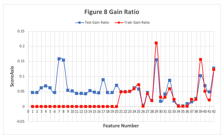
Another attempt was made using Python, please see Appendix B for the code snippet (Van Ede 2018). The values of the results produced do not agree with those presented in the Evaluation Paper but the shape and trend is somewhat similar. It is difficult to determine why the absolute values do not agree as there is no information in the Evaluation Paper about how the algorithm was implemented.
The Gain Ratios for the UNSW-NB15-Testing set and part of the training set are presented in Figure 8 below and Appendix F, each feature was taking hours to calculate and 1 to 20 in the train set did not complete in time. The results do show that some features have a relatively high Information Gain and low Gain Ratio but that is more due to the number of distinct values in the feature rather than its correlation with the label. In the Evaluation Paper the Gain Ratios for the features in the testing and training sets are also similar.
3.2 Machine Learning Models
Visual Studio Business Intelligence 2008 was used in the Evaluation Paper but it is no longer supported by Microsoft. The tools used in this work were Visual Studio 2019 (Visual Studio 2019), SQL Server 2019 (SQL Server 2019) and the SQL Server Analysis Services (SSAS) from the Microsoft Analysis Services 2020 library (Microsoft Analysis Services 2020).
Five ML models were used to evaluate the complexity of the UNSW datasets and to compare the results to the KDDCUP1999 data set. The specific data sets and features used are detailed in Tables 1, 2 and 3. Please see Appendix I and J which shows the Visual Studio Mining Structure and the SQL Server structure.
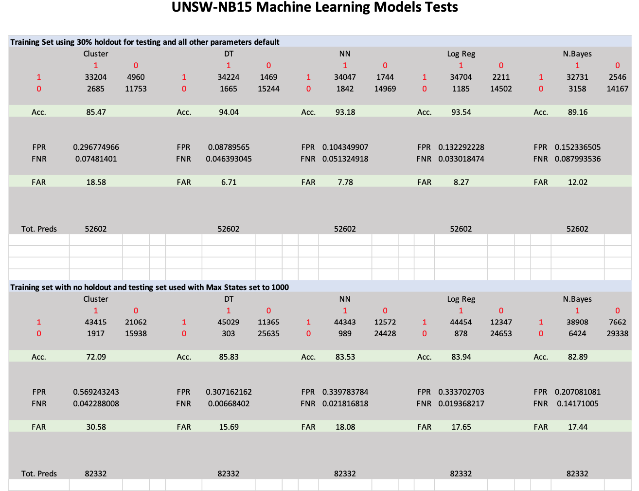
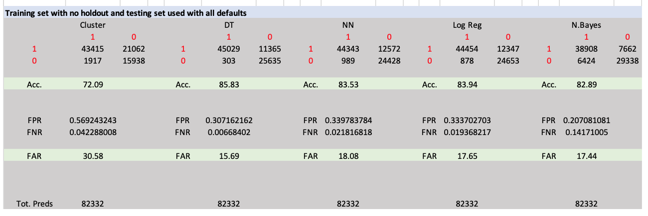
The five models used are Naïve Bayes (NB), Decision Tree (DT), Neural Network (NN), Logistic Regression (LR) and Clustering. The authors did not provide enough information to implement the models such that the results could be exactly reproduced with the newer tools. Three sets of tests were run on the UNSW-NB15 data sets with varying parameters and two sets of tests were run on the KDDCUP1999 data sets.
In the Evaluation Paper the accuracy is defined as:
(True Positive + True Negative) /
(True Positive + True Negative + False Positive + False Negative).
In the Evaluation Paper the False Alarm Rate (FAR) is defined by:
False Positive Rate (FPR) = False Positive / (False Positive + True Negative) False Negative Rate (FNR) = False Negative / (False Negative + True Positive) FAR is given by (FPR + FNR) / 2
3.3 SVM and NN Models
The data set used for training and testing the SVM and NN was the UNSW-NB15_1.csv which contains 700,001 records and is a simple split of the entire set of records. It is not curated like the training and testing sets used in the above analysis; it only has 22,215 attack records but is more a reflection of the raw network data flow. The features used in the previously analysis were used here with the same mappings between strings and integers using the SPSS transform tool. Consideration was given to using the source and destination IP and Port fields but after closer examination it appears that the malicious traffic stems from one or two addresses so using these features would be essentially putting a label on the records, that is IP address X equals malicious traffic.
3.4.0 SVM
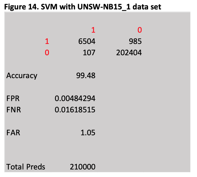
R Studio was used to implement the SVM please see Appendix C for the code. The trainControl function was used with method set to CV and number set to 5, during training this splits the training data into 5 sets and uses each set as testing data for the model trained on the other 4 sets. This 5-fold cross validation estimates the prediction error by taking the average of the error across all tests. The preProcess function was used with the parameters set to centre and scale which standardise the data so that the features have a mean value of 0 and a standard deviation of 1. The tuneLength parameter was set to 5 and this allows the model to choose 5 different sets of parameters to determine the optimum for the data set. 30% of the data was held out for testing.
The results are presented below in Figure 14 and using the definition of accuracy and FAR outlined in section 3.3 the SVM achieves an accuracy of 99.48% and a FAR of 1.05%
3.4.1 Neural Network
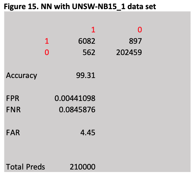
Using the same data set and features as outlined for the SVM a NN was implemented in Visual Studio 2019 SSAS. Two of the Mining Structure parameters were changed, HoldoutMaxPercent was set to 30 and the HoldoutSeed was set to 1. Two of the Neural Network Algorithm parameters were changed, MAXIMUM_STATES was set to 1000 and SAMPLE_SIZE was set to 700,000 * 0.7.
The results are presented below in Figure 15 and using the definition of accuracy and FAR outlined in section 3.3 the NN achieves an accuracy of 99.31% and a FAR of 4.45%
4.0 Results
Excluding Gain Ratio, the statistic and correlation tests as presented in the Evaluation Paper were repeatable and do show that the features of the train and test set are statistically very similar and can be used to reliably evaluate the five ML models.
The five SSAS ML models used provided results that agreed with those reported in the Evaluation Paper. The results that most agreed were obtained when using the training set with no holdout, the testing set used for testing and the mining structure and mining model MAX-STATES parameter was changed to 1000.
Both the tuned SVM and NN achieved very high accuracies and very low FAR percentages but the false alarms still numbered in the hundreds and would be considered unacceptable by any Network Administrator.
One idea that occurs to me and is an area of research that could be pursued further is the notion of using ML models in a series and or parallel pipeline where the results from some select models run in parallel are cross checked with each other before being piped into a final output model.
5.0 Conclusions
Except for the Gain Ratio analysis, the results obtained agree with those presented in the Evaluation Paper and confirm that the UNSW-NB15 data set is more complex than the KDDCUP1999 data set. Even though the SVM achieved an accuracy of 99.48% depending on the size of the network it may only take minutes to observe hundreds of thousands of packets traversing the network so 985 false positives and 107 false negatives from a test of 210, 000 would be considered unacceptable by any Network Administrator. The results show that the UNSW-NB15 data set is suitable for developing models to detect anomalous network traffic, but the statistical analysis and ML models used in the Evaluation Paper and extended in this work could only be considered a starting point in terms of developing sophisticated classifiers with very low numbers of false alarms that could be used in a production environment.
References
Brownlee, J. (2020) Information Gain and Mutual Information for Machine Learning. Retrieved from https://machinelearningmastery.com/information-gain-and-mutual-information/
KDDCUP1999. (2007). Retrieved from http://kdd.ics.uci.edu/databases/kddcup99/kddcup99.html
MatLab tool. (2020). Retrieved from https://au.mathworks.com/products/matlab.html
Microsoft Analysis Services. 2020. (2020). Retrieved from https://marketplace.visualstudio.com/items?itemName=ProBITools.MicrosoftAnalysisServicesModelingProjects
Mohammed, M., Badruddin, M. K., Bashier, E.B.M. (2016). Machine Learning: Algorithms and Applications. (pp. 44-52). CRC Press.
Moustafa, N., & Slay, J. (2016). The evaluation of Network Anomaly Detection Systems: Statistical analysis of the UNSW-NB15 data set and the comparison with the KDD99 data set. Information Security Journal: A Global Perspective, 25(1-3), 18-31.
Moustafa, N. (2018). The UNSW-NB15 Dataset Description. Retrieved from https://www.unsw.adfa.edu.au/unsw-canberra-cyber/cybersecurity/ADFA-NB15-Datasets/
SPSS tool. (2020). Retrieved from https://www.ibm.com/analytics/spss-statistics-software
SQL Server 2019. (2019). Retrieved from https://www.microsoft.com/en-us/sql-server/sql-server-downloads
Van Ede, T. (2018). info-gain. Retrieved from https://github.com/Thijsvanede/info_gain
Visual Studio 2019. (2019). Retrieved from https://visualstudio.microsoft.com/downloads/